Regression Analysis

Data Distribution

happy_df = readxl::read_xls('DataPanelWHR2021C2.xls') %>% 
  janitor::clean_names() %>% 
  rename("happiness_score"= life_ladder)

To identify the significance of relationships and establish a regression model to predict the happiness score, we first take a look on the distribution of each variable.

par(mfrow= c(3,3))
for (n in 3:ncol(happy_df)){
  var = names(happy_df)[n] %>% 
    str_replace_all("_"," ") %>% 
    str_to_title()
  pull(happy_df,n) %>% 
    hist(main=NA,xlab=var)
}
mtext("Variable Distribution", side = 3, line = -2, outer = TRUE)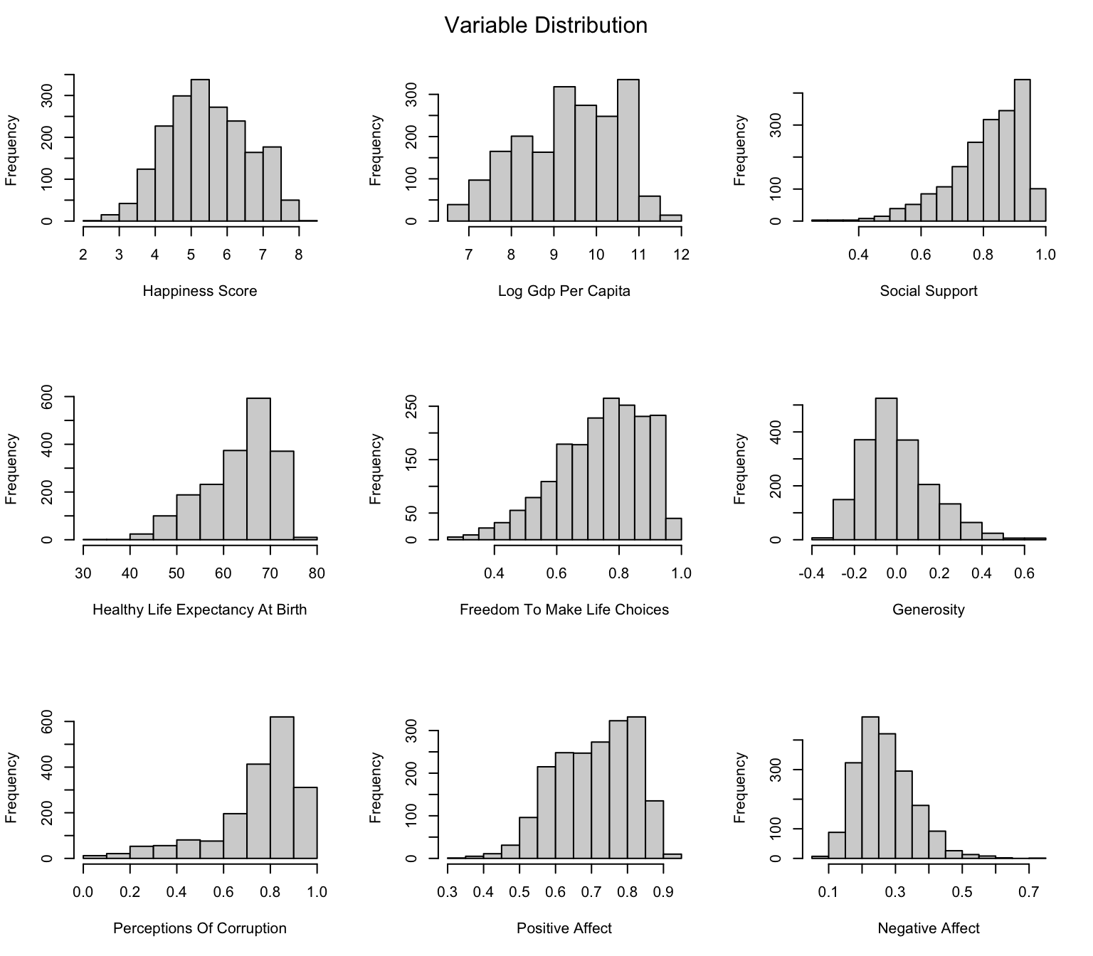

Here our happiness score follows great bell shape and is relatively non-skewed. Most of the factors are normally distributed. Therefore we can proceed to build regression model.

Linear regression model

Since all factors are continuous, we can apply fundamental linear regression here.

# General Model
happy_fit = happy_df %>% 
  select(-country_name,-year)
fit = happy_fit %>%
  lm(happiness_score~., data=.)
fit_est = fit %>% 
  broom.mixed::tidy() %>% 
  mutate(
    term = str_replace_all(term,"_"," "),
    term = str_to_title(term))

knitr::kable(fit_est)

term	estimate	std.error	statistic	p.value
(Intercept)	-2.5253237	0.1862968	-13.5553776	0.0000000
Log Gdp Per Capita	0.3823714	0.0254857	15.0034000	0.0000000
Social Support	1.8444740	0.1752311	10.5259501	0.0000000
Healthy Life Expectancy At Birth	0.0267282	0.0034677	7.7078655	0.0000000
Freedom To Make Life Choices	0.3900271	0.1307944	2.9819865	0.0029046
Generosity	0.4195941	0.0923454	4.5437459	0.0000059
Perceptions Of Corruption	-0.6997192	0.0879900	-7.9522603	0.0000000
Positive Affect	1.9879308	0.1700964	11.6870863	0.0000000
Negative Affect	0.1853176	0.1865965	0.9931458	0.3207803

The result indicated that Log Gdp Per Capita, Social Support, Healthy Life Expectancy At Birth, Freedom To Make Life Choices, Generosity, Perceptions Of Corruption, Positive Affect are all significantly correlated with happiness score, while Negative Affect does not.

Model diagnostic

To test if the model follows assumption of normal distribution, we could plot the QQ plots and related diagnostic plots.

par(mfrow=c(2,2))
plot(fit)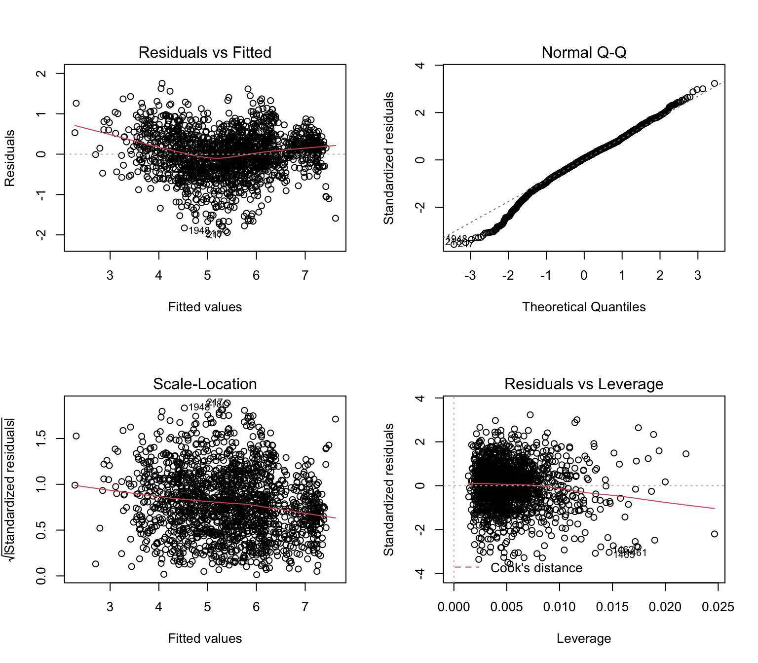

The majority of data follows normal distribution, thus we could go on.

Cross Validation

To test the model efficiency and its predictory ability, we apply 100 times of cross validation and calculate the mean value of root mean squared errors (RMSE) over 100 CVs.

set.seed(1)

cv_df = crossv_mc(happy_fit, 100) %>% 
  mutate(train = map(train,as_tibble),
         test = map(test, as_tibble)) %>% 
  mutate(linear_mod = map(train, ~lm(happiness_score ~ ., data = .x)) ) %>% 
  mutate(
    rmse_linear = map2_dbl(linear_mod, test, ~rmse(model = .x, data = .y)) )

ggplot(cv_df,aes(x="linear",y=rmse_linear)) +
  geom_violin(fill="lightblue",alpha=0.7) +
  labs(x = NULL, y = "RMSE",title = "RMSE of Linear Model Cross-Validation")+
  theme_bw()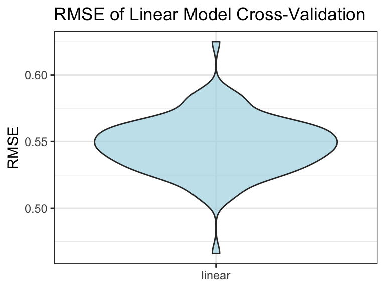

mean_rmse = mean(pull(cv_df,rmse_linear))

Here we can see the mean RMSE is 0.5472725, which is acceptable. Therefore, the model could be used to predict the country’s happiness score.

Model Interpretation

The outcome of the project suggests that happiness has positive associations with GDP per capita in purchasing power parity, social support, healthy life expectancy at birth, national average freedom to make life choices, generosity, positive affect measures (happiness, laugh, and enjoyment), while happiness has negative associations with negative affect measures (worry, sadness and anger) and national corruption.